52-Week Low Quality: Global Comparison Across 16 Exchanges
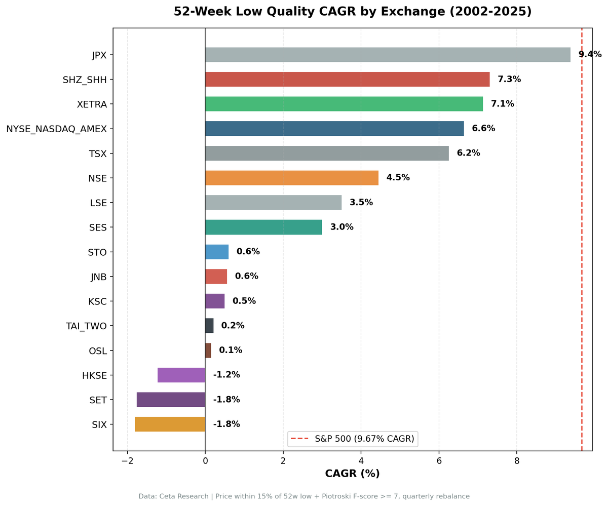
We tested the 52-Week Low + Piotroski F-score strategy across 16 global exchanges from 2002 to 2025. Five beat their local benchmark. Japan and China lead on raw excess; Germany is the most defensive implementation.

The strategy is straightforward: buy financially healthy stocks that are near their annual lows, wait for them to recover, rotate quarterly. Simple premise. The question is whether the premise holds globally or just in certain market structures.
Contents
- Method
- What We Found
- Why China, Japan, and Germany Work
- The US Paradox
- Where the Strategy Structurally Fails
- The Down-Capture Story
- Run It Yourself
- Limitations
We ran this screen on 16 exchanges covering 2002-2025, each measured against its local benchmark (Sensex for India, DAX for Germany, Nikkei for Japan, etc.). The results range from +3.56% annual excess in China to -10.76% in Norway. Three exchanges beat their local benchmark cleanly, two more roughly match it. The rest underperform, some catastrophically.
Here's the full picture.
Data: FMP financial data warehouse, 2000–2025. Updated August 2026 with next-day-close execution and data-quality guards.
Method
Every quarter (January, April, July, October), screen stocks trading within 15% of their 52-week low with a Piotroski F-score of 7 or higher. The Piotroski filter requires improving profitability, leverage, and efficiency, it removes companies that are cheap for fundamental reasons. Hold up to 30 stocks equal-weight, minimum 5 to deploy capital. Costs: 0.1% per trade. Filing lag: 45 days. Execution: next-day close (market-on-close).
Each exchange is benchmarked against its local index (Sensex, DAX, Nikkei, TSX Composite, etc.) to measure alpha in local currency terms. This is the correct comparison for a local investor.
These benchmarks leave dividends out. Portfolio returns here use dividend-adjusted prices, so they include dividends. Most of the indices we measure against do not. The FTSE 100, Hang Seng, KOSPI, Nikkei 225, OMX Stockholm 30, Oslo All Share, SET Index, SMI, SSE Composite, STI, Sensex, TAIEX and TSX Composite are price indices, so excess return against them is overstated by roughly the local dividend yield, which has run between about 1.3% and 3.5% in these markets. Those comparisons are like for like: the S&P 500 figure runs through SPY, which is dividend-adjusted; the DAX is a performance index. Treat any edge thinner than the local yield as a tie rather than a win.
What We Found
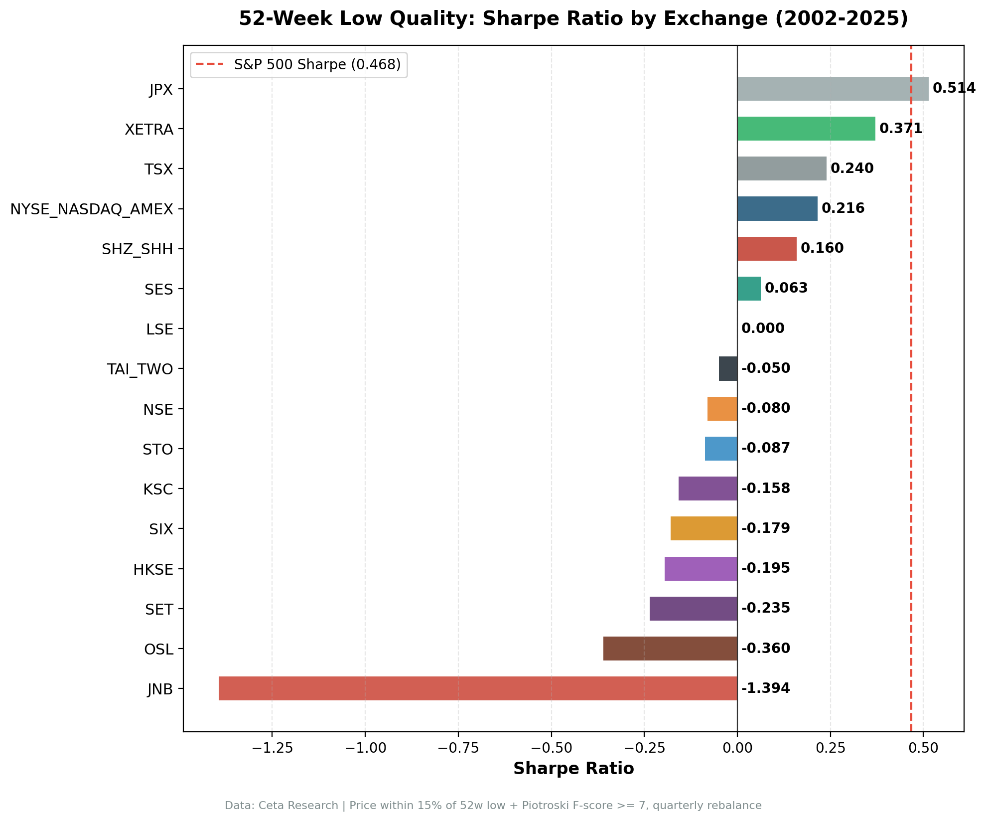
| Exchange | CAGR | Benchmark | vs Local | Sharpe | MaxDD | Dn-Cap | Cash% | Avg Stks |
|---|---|---|---|---|---|---|---|---|
| JPX (Japan) | 9.38% | Nikkei 6.16% | +3.23% | 0.514 | -48.08% | 55.6% | 4% | 25.5 |
| SHZ+SHH (China) | 7.30% | SSE 3.74% | +3.56% | 0.160 | -54.56% | 76.7% | 9% | 26.8 |
| XETRA (Germany) | 7.13% | DAX 6.76% | +0.37% | 0.371 | -30.5% | 35.4% | 2% | 23.9 |
| US (NYSE+NASDAQ+AMEX) | 6.64% | S&P 500 9.67% | -3.03% | 0.216 | -48.17% | 112.6% | 0% | 28.4 |
| TSX (Canada) | 6.25% | TSX Comp 5.95% | +0.30% | 0.240 | -37.11% | 74.0% | 9% | 20.5 |
| India (NSE) | 4.45% | Sensex 14.48% | -10.03% | -0.08 | -56.09% | 75.8% | 34% | 21.6 |
| LSE (UK) | 3.50% | FTSE 2.52% | +0.98% | 0.000 | -46.72% | 8% | 19.9 | |
| SES (Singapore) | 3.00% | STI 4.20% | -1.20% | 0.063 | -17.1% | 66% | 8.8 | |
| STO (Sweden) | 0.60% | OMX30 5.09% | -4.49% | -0.087 | -60.2% | 56% | 15.2 | |
| JNB (South Africa) | 0.56% | SPY** 9.67% | -9.11% | -1.394 | -20.77% | 87% | 7.3 | |
| KSC (Korea) | 0.50% | KOSPI 6.92% | -6.41% | -0.158 | -40.7% | 53.6% | 39% | 21.2 |
| TAI+TWO (Taiwan) | 0.21% | TAIEX 6.74% | -6.53% | -0.05 | -48.64% | 31% | 23.5 | |
| OSL (Norway) | 0.15% | Oslo AS 10.91% | -10.76% | -0.36 | -19.23% | 88%* | 7.4 | |
| HKSE (Hong Kong) | -1.22% | Hang Seng 3.76% | -4.99% | -0.195 | -75.78% | 82.0% | 15% | 22.8 |
| SET (Thailand) | -1.76% | SET 6.25% | -8.01% | -0.235 | -60.36% | 41% | 20.1 | |
| SIX (Switzerland) | -1.81% | SMI 2.85% | -4.66% | -0.179 | -62.86% | 58.6% | 36% | 17.9 |
Norway's cash share (88%) is over all 95 rebalances; metrics use only the 50 quarters where the Oslo All Share has FMP data. *JNB falls back to SPY because no local index data is available in FMP.
Three exchanges beat their local benchmark cleanly: China (+3.56%), Japan (+3.23%), and the UK (+0.98%). Germany (+0.37%) and Canada (+0.30%) roughly match theirs; edges that thin are within rerun noise. The rest underperform, some severely.
Why China, Japan, and Germany Work
China leads on raw excess: 7.30% CAGR, +3.56% vs the SSE Composite, Sharpe 0.160, alpha +3.95%. The Sharpe is modest because Chinese A-shares run at 30% volatility, but the absolute outperformance over 24 years is real. Win rate above 50%. The quality filter does meaningful work in a retail-dominated market where fundamentals are routinely mispriced.
Japan is the next-strongest result: 9.38% CAGR, +3.23% vs the Nikkei 225, Sharpe 0.514, alpha +5.01%. Previously excluded from this study due to insufficient FY data, JPX now has enough coverage to run the full backtest. Only 4 cash periods in 95 quarters. Win rate of 56.84%, the highest of any exchange.
Japan's equity market shares structural similarities with Germany. The Tokyo Stock Exchange is dominated by precision manufacturers, automotive suppliers, electronics companies, and trading houses. These businesses have genuine earnings cycles. They trade near 52-week lows when exports slow or the yen strengthens. With Piotroski scores of 7+, they're operationally sound. When the headwind fades, they recover.
Germany now sits at 7.13% CAGR, +0.37% vs the DAX, Sharpe 0.371, alpha +2.9%. Max drawdown of -30.5% vs the DAX's -51.25%. The down-capture of 35.4% is the best in the table: when the DAX falls, this portfolio absorbs roughly a third of the loss. The raw excess is thinner than earlier (uncorrected) backtests showed, but Germany remains the most defensive implementation we found.
The XETRA composition explains this. Mittelstand-adjacent industrials, specialty chemicals, automotive suppliers, capital equipment companies. These businesses are genuinely cyclical. They trade near 52-week lows when order books dry up during slowdowns. They have strong Piotroski scores because their underlying business models are sound. And they mean-revert cleanly when the cycle turns.
All three share three conditions: (1) cyclical or sentiment-driven name flow into the screen, (2) accounting that makes the Piotroski filter meaningful, and (3) lower algo saturation than the US means the signal has time to play out at quarterly frequency.
The US Paradox
The US result is the most instructive failure. Zero cash periods, the market always had qualifying stocks. 6.64% CAGR vs SPY's 9.67%, a -3.03% annual drag. Down-capture of 112.6%.
The explanation: the US market is the most efficiently priced in the world. When a US stock drops to its 52-week low, thousands of analysts, quant funds, and algorithmic traders have already noticed. The mean-reversion signal gets arbitraged away before a quarterly rebalancing strategy can capture it. The 52-week-low discount exists, but it evaporates fast. By the time the screen fires and you buy, much of the recovery is already priced in.
The 112.6% down-capture is the other side of this problem. In US corrections, there's no flight to safety in beaten-down value stocks. Everything falls together. Liquidity and market depth mean these names correlate tightly with the index during risk-off episodes.
Canada (TSX) roughly matches its local benchmark at 6.25% CAGR vs TSX Composite's 5.95%. That +0.30% excess is within noise of par, call it a wash. Canadian equities have more exposure to materials and energy companies, genuinely cyclical businesses where the mean-reversion mechanism at least doesn't lose ground.
Where the Strategy Structurally Fails
Three exchanges are effectively unusable: Norway (88% cash), Singapore (66% cash), and South Africa (87% cash).
Norway's Sharpe of -0.36 is among the worst in the table. But the cash rate tells the real story. 88% of quarters had fewer than 5 qualifying stocks. The Oslo Bors is heavily weighted toward energy and shipping. The Piotroski screen is demanding, energy companies near lows often have deteriorating cash flows and leverage metrics. The screen correctly avoids them, but that means the strategy mostly sits idle. The Oslo All Share returned 10.91% annually, making the -10.76% excess gap enormous.
Singapore returned 3.00% CAGR vs the STI's 4.20%. 66% cash means you're earning money market rates for two-thirds of the test period. The exchange is too thin for this strategy.
South Africa has a -1.394 Sharpe, the worst absolute risk-adjusted number in the table. The 87% cash rate combined with extreme tail returns when it does invest is a brutal combination.
The Down-Capture Story
Down-capture is the metric that separates useful strategies from expensive index tracking. With local benchmarks, the picture changes:
| Exchange | Benchmark | Down-Capture |
|---|---|---|
| Germany (XETRA) | DAX | 35.4% |
| Japan (JPX) | Nikkei | 55.6% |
| Canada (TSX) | TSX Comp | 74.0% |
| India (NSE) | Sensex | 75.8% |
| China (SHZ+SHH) | SSE Composite | 76.7% |
| Hong Kong (HKSE) | Hang Seng | 82.0% |
| US | S&P 500 | 112.6% |
Germany's 35.4% down-capture vs the DAX is the standout. When the DAX falls, this portfolio absorbs roughly a third of the loss. Combined with +0.37% excess CAGR and a -30.5% max drawdown vs the DAX's -51.25%, that's genuine risk-adjusted outperformance.
Japan's 55.6% down-capture vs the Nikkei is solid but less dramatic. The +3.23% excess more than compensates. Japan is the highest absolute CAGR (9.38%) of any exchange in the test.
China now shows +3.56% excess vs the SSE Composite, the highest local excess in the table. The Sharpe of 0.160 is modest, but the strategy does generate genuine local alpha in a market where retail sentiment dominates and fundamental quality is underpriced.
Germany and Japan are the two exchanges combining genuine crash protection with positive excess returns vs local benchmarks. China leads on raw CAGR excess but with much higher volatility. Everything else involves a meaningful trade-off.
Run It Yourself
The query below screens all supported exchanges simultaneously. Filter by exchange column to isolate specific markets.
WITH
inc AS (
    SELECT symbol, netIncome, grossProfit, revenue,
           ROW_NUMBER() OVER (PARTITION BY symbol ORDER BY dateEpoch DESC) AS rn
    FROM income_statement WHERE period = 'FY' AND netIncome IS NOT NULL
),
bal AS (
    SELECT symbol, totalAssets, totalCurrentAssets, totalCurrentLiabilities,
           longTermDebt, totalStockholdersEquity,
           ROW_NUMBER() OVER (PARTITION BY symbol ORDER BY dateEpoch DESC) AS rn
    FROM balance_sheet WHERE period = 'FY' AND totalAssets > 0
),
cf AS (
    SELECT symbol, operatingCashFlow,
           ROW_NUMBER() OVER (PARTITION BY symbol ORDER BY dateEpoch DESC) AS rn
    FROM cash_flow_statement WHERE period = 'FY' AND operatingCashFlow IS NOT NULL
),
piotroski AS (
    SELECT ic.symbol,
        CASE WHEN ic.netIncome > 0 THEN 1 ELSE 0 END
        + CASE WHEN cfc.operatingCashFlow > 0 THEN 1 ELSE 0 END
        + CASE WHEN (ic.netIncome/bc.totalAssets) > (ip.netIncome/bp.totalAssets) THEN 1 ELSE 0 END
        + CASE WHEN cfc.operatingCashFlow/bc.totalAssets > ic.netIncome/bc.totalAssets THEN 1 ELSE 0 END
        + CASE WHEN (COALESCE(bc.longTermDebt,0)/bc.totalAssets) < (COALESCE(bp.longTermDebt,0)/bp.totalAssets) THEN 1 ELSE 0 END
        + CASE WHEN (bc.totalCurrentAssets/bc.totalCurrentLiabilities) > (bp.totalCurrentAssets/bp.totalCurrentLiabilities) THEN 1 ELSE 0 END
        + CASE WHEN bc.totalStockholdersEquity >= bp.totalStockholdersEquity THEN 1 ELSE 0 END
        + CASE WHEN (ic.revenue/bc.totalAssets) > (ip.revenue/bp.totalAssets) THEN 1 ELSE 0 END
        + CASE WHEN (ic.grossProfit/ic.revenue) > (ip.grossProfit/ip.revenue) THEN 1 ELSE 0 END
        AS f_score
    FROM (SELECT * FROM inc WHERE rn=1) ic
    JOIN (SELECT * FROM inc WHERE rn=2) ip ON ic.symbol = ip.symbol
    JOIN (SELECT * FROM bal WHERE rn=1) bc ON ic.symbol = bc.symbol
    JOIN (SELECT * FROM bal WHERE rn=2) bp ON ic.symbol = bp.symbol
    JOIN (SELECT * FROM cf WHERE rn=1) cfc ON ic.symbol = cfc.symbol
),
prices_52w AS (
    SELECT symbol,
           LAST_VALUE(adjClose) OVER (PARTITION BY symbol ORDER BY dateEpoch ROWS BETWEEN UNBOUNDED PRECEDING AND UNBOUNDED FOLLOWING) AS current_price,
           MIN(adjClose) OVER (PARTITION BY symbol) AS low_52w
    FROM stock_eod
    WHERE CAST(date AS DATE) >= CURRENT_DATE - INTERVAL '365 days' AND adjClose > 0
),
price_summary AS (
    SELECT symbol, MAX(current_price) AS current_price, MIN(low_52w) AS low_52w
    FROM prices_52w GROUP BY symbol
)
SELECT pio.symbol, p.companyName, p.exchange, p.sector,
       pio.f_score,
       ROUND(ps.current_price, 2) AS current_price,
       ROUND(ps.low_52w, 2) AS low_52w,
       ROUND((ps.current_price - ps.low_52w)/ps.low_52w * 100, 1) AS pct_above_low,
       ROUND(p.marketCap/1e9, 2) AS mktcap_b
FROM piotroski pio
JOIN profile p ON pio.symbol = p.symbol
JOIN price_summary ps ON pio.symbol = ps.symbol
JOIN key_metrics_ttm k ON pio.symbol = k.symbol
WHERE p.marketCap > 100000000
  AND pio.f_score >= 7
  AND (ps.current_price - ps.low_52w)/ps.low_52w <= 0.15
  AND ps.current_price >= 1.0
  AND p.isFund = false
  AND p.isEtf = false
  AND p.isActivelyTrading = true
QUALIFY ROW_NUMBER() OVER (PARTITION BY p.companyName
                           ORDER BY p.averageVolume DESC) = 1
ORDER BY (ps.current_price - ps.low_52w)/ps.low_52w ASC
LIMIT 30
Run the live global screen on Ceta Research Data Explorer.
Limitations
Local benchmarks are the correct comparison. Each exchange uses its local index (DAX, Sensex, Nikkei, etc.) rather than SPY. This measures alpha in the currency and market structure relevant to a local investor. The trade-off: cross-exchange comparison is harder when each benchmark is different.
Currency effects: All returns are in local currency. Exchange rates matter for international investors. The Swiss franc's safe-haven appreciation, the Indian rupee's depreciation, and the HKD's USD peg all affect USD-denominated returns differently.
Survivorship bias: Delisted companies are excluded across all exchanges. This effect is most pronounced in markets with high delistings (Hong Kong 2020-2024, emerging markets generally). Results are modestly overstated in those markets.
Period dependency: 2002-2025 includes two global crashes, a long QE-driven bull market, and a tech-led recovery. Results from other 24-year windows would differ. Japan's outperformance and Germany's defensive profile hold across sub-periods; other results are more period-sensitive.
Market structure changes: The strategy's performance in some exchanges (Hong Kong, China) reflects regime changes not present in the backtest's early years. Mean-reversion assumptions break down when market structure shifts.
The bottom line: this strategy has three implementations worth running, JPX (Japan), SHZ+SHH (China), and XETRA (Germany). Japan and China beat their local benchmarks; Germany roughly matches the DAX but with the best defensive profile in the test (35.4% down-capture, -30.5% max drawdown). China leads on raw excess CAGR at the cost of 30% volatility. The rest are either structural misfits (too few qualifying stocks) or markets where the mean-reversion mechanism doesn't hold.
Data: Ceta Research (FMP financial data warehouse), 2002–2025. Each exchange benchmarked against its local index in local currency. Full methodology: METHODOLOGY.md. Backtest code: backtests/52-week-low/. Past performance does not guarantee future results. This is educational content, not investment advice.