Low Volatility + Quality: 0.484 Sharpe vs 0.361 for the S&P 500 Over 25 Years
We backtested a low-volatility quality screen on US stocks (NYSE, NASDAQ, AMEX) from 2000 to 2025. It delivered 6.53% CAGR with a 0.484 Sharpe vs 0.361 for the S&P 500, a -26.0% max drawdown vs -43.9%, and captured only 27% of market downside. Boring stocks, better risk-adjusted returns.

Finance textbooks say take more risk, earn more return. Fifty years of data say otherwise. We screened for the 30 lowest-volatility quality stocks on US exchanges and backtested from 2000 to 2025 using next-day execution prices. The portfolio returned 6.53% CAGR with a 0.484 Sharpe ratio, beating the S&P 500's 0.361. Max drawdown was -26.0% vs -43.9% for the benchmark. The strategy captured only 27% of market downside while participating in 50% of market upside.
Contents
- Method
- What Research Shows
- The Screen
- Simple Screen (Quality Filter Only)
- Advanced Screen (Quality + Volatility Concept)
- Results
- When It Works
- When It Struggles
- Full Annual Returns
- Limitations
- Global Results
- Run It Yourself
- Takeaway
- References
The absolute CAGR is lower than the S&P 500. That's the trade-off. You give up some upside for dramatically less risk. For investors who care about risk-adjusted returns, drawdown protection, and capital preservation, that's a good deal.
Data: FMP financial data warehouse, 2000–2025. Updated March 2026.
Method
Data source: Ceta Research (FMP financial data warehouse, 70K+ global stocks) Universe: All US stocks on NYSE, NASDAQ, AMEX with market cap > $1B Period: January 2000 to March 2025 (25.8 years, 103 quarterly periods) Rebalancing: Quarterly (January, April, July, October) Benchmark: S&P 500 (SPY) Cash rule: Portfolio holds cash if fewer than 10 stocks qualify Transaction costs: Size-tiered model (0.1% for large caps, 0.3% for mid caps, 0.5% for small caps) Data quality guards: 45-day lag on annual filings, minimum 200 trading days for vol computation, max single return capped at 200%, penny stocks (< $1) excluded
Signal filters:
| Filter | Threshold | Source |
|---|---|---|
| Return on equity | > 10% | key_metrics FY |
| Operating profit margin | > 10% | financial_ratios FY |
| Market cap | > $1B | key_metrics FY |
| 252-day realized volatility | Rank ASC, top 30 | stock_eod daily returns |
| Minimum trading days | >= 200 in 14-month window | stock_eod |
What Research Shows
The low-volatility anomaly is one of the most robust findings in empirical finance.
Ang, Hodrick, Xing and Zhang (2006) sorted US stocks by volatility from 1963 to 2000. The most volatile stocks earned far lower risk-adjusted returns than the least volatile, a gap of roughly 1% per month. In follow-up work, the same authors (2009) documented the same pattern across 23 developed markets. Same result everywhere.
Baker, Bradley and Wurgler (2011) explained why. Fund managers measured against the S&P 500 avoid low-vol stocks because the resulting portfolio has high tracking error. Even if a low-vol portfolio has a better Sharpe ratio, the manager looks bad when the benchmark rallies. This creates persistent neglect of low-beta stocks.
Frazzini and Pedersen (2014) added leverage constraints to the story. Investors who can't borrow buy high-beta stocks to reach return targets. This bids up high-beta prices and compresses their returns while leaving low-beta stocks underpriced.
Adding quality filters matters. Novy-Marx (2013) showed gross profitability is a strong return predictor independent of value. Our quality overlay (ROE > 10%, operating margin > 10%) removes companies that are "low volatility because dying." A stock flatlined at $2 with declining revenue has low vol but no investment merit. Quality filters keep the "boring and good" stocks and remove the "boring and dying" ones.
The Screen
Simple Screen (Quality Filter Only)
SELECT
  k.symbol,
  p.companyName,
  ROUND(k.returnOnEquityTTM * 100, 2) AS roe_pct,
  ROUND(f.operatingProfitMarginTTM * 100, 2) AS opm_pct,
  ROUND(k.marketCap / 1e9, 2) AS mktcap_b
FROM key_metrics_ttm k
JOIN financial_ratios_ttm f ON k.symbol = f.symbol
JOIN profile p ON k.symbol = p.symbol
WHERE k.returnOnEquityTTM > 0.10
  AND f.operatingProfitMarginTTM > 0.10
  AND k.marketCap > 1000000000
  AND p.exchange IN ('NYSE', 'NASDAQ', 'AMEX')
  AND p.country = 'US'
  AND p.isFund = false
  AND p.isEtf = false
ORDER BY k.marketCap DESC
LIMIT 30
This produces the quality universe. The full strategy ranks these candidates by trailing 252-day volatility (computed from daily returns) and selects the 30 lowest-volatility names.
Advanced Screen (Quality + Volatility Concept)
Computing realized volatility requires daily price data. The backtest computes STDDEV(daily log returns) * SQRT(252) over a 14-month lookback window. This can't be done in a single SQL query against the FMP warehouse since it requires processing daily prices for each symbol.
The quality filter is the actionable screen. Volatility ranking is applied in the backtest code.
Try the quality screen on Ceta Research
Results
| Metric | Low Vol + Quality | S&P 500 |
|---|---|---|
| CAGR | 6.53% | 8.02% |
| Total Return | 410.0% | 628.3% |
| Max Drawdown | -26.0% | -43.9% |
| Annualized Volatility | 9.36% | 16.68% |
| Sharpe Ratio | 0.484 | 0.361 |
| Sortino Ratio | 0.778 | 0.536 |
| Calmar Ratio | 0.251 | 0.183 |
| VaR (95%) | -5.89% | -14.62% |
| Beta | 0.396 | 1.0 |
| Alpha | 2.15% | -- |
| Up Capture | 50.4% | -- |
| Down Capture | 27.5% | -- |
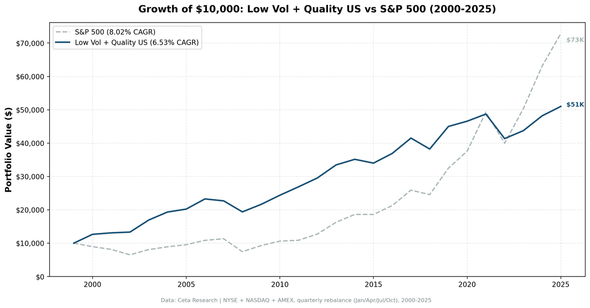
$10,000 invested in 2000 grew to $51,003 in the low-vol quality portfolio vs $72,830 in SPY. The S&P 500 produced higher absolute returns. But the low-vol portfolio achieved this with 44% less volatility, 41% smaller max drawdown, and a Sharpe ratio that's 34% higher.
The capture ratio tells the story: 50% up capture vs 27% down capture. The portfolio participates in half the market's gains but avoids nearly three-quarters of its losses. Over 25 years, that asymmetry compounds into better risk-adjusted returns.
When It Works
Bear markets. The strategy's biggest edge comes when markets fall.
| Year | Low Vol + Quality | S&P 500 | Excess |
|---|---|---|---|
| 2000 | +26.5% | -10.5% | +37.0% |
| 2002 | +1.8% | -19.9% | +21.7% |
| 2008 | -14.6% | -34.3% | +19.8% |
| 2011 | +10.4% | +2.5% | +7.9% |
During the dot-com crash, the portfolio gained 27% while SPY lost 10%. In 2008, it fell 15% while SPY fell 34%. The quality filter keeps profitable companies, and low vol means these stocks drop less when fear spikes.
Flat markets. In years like 2011 (SPY +2.5%), the portfolio returned 10.4%. Low-vol stocks compound steadily without the sharp drawdowns that destroy long-term returns.
When It Struggles
Momentum rallies. When risk-seeking dominates, low-vol stocks lag badly.
| Year | Low Vol + Quality | S&P 500 | Excess |
|---|---|---|---|
| 2021 | +4.6% | +31.3% | -26.7% |
| 2023 | +5.7% | +26.0% | -20.3% |
| 2019 | +17.7% | +32.3% | -14.6% |
| 2020 | +3.5% | +15.6% | -12.1% |
2021 was the worst year: SPY returned 31% driven by speculative growth. Low-vol quality stocks returned 4.6%. The Magnificent Seven and meme stock mania rewarded exactly the kind of stocks this strategy avoids.
This is the strategy working as designed. It avoids overvalued, high-beta names. But during manias, that looks like underperformance.
Full Annual Returns
| Year | Low Vol + Quality | S&P 500 | Excess |
|---|---|---|---|
| 2000 | +26.5% | -10.5% | +37.0% |
| 2001 | +3.5% | -9.2% | +12.7% |
| 2002 | +1.8% | -19.9% | +21.7% |
| 2003 | +27.1% | +24.1% | +3.0% |
| 2004 | +14.1% | +10.2% | +3.9% |
| 2005 | +4.5% | +7.2% | -2.6% |
| 2006 | +15.1% | +13.7% | +1.5% |
| 2007 | -2.5% | +4.4% | -6.9% |
| 2008 | -14.6% | -34.3% | +19.8% |
| 2009 | +11.6% | +24.7% | -13.2% |
| 2010 | +12.7% | +14.3% | -1.6% |
| 2011 | +10.4% | +2.5% | +7.9% |
| 2012 | +9.8% | +17.1% | -7.3% |
| 2013 | +13.2% | +27.8% | -14.5% |
| 2014 | +5.0% | +14.5% | -9.4% |
| 2015 | -3.3% | -0.1% | -3.1% |
| 2016 | +8.6% | +14.4% | -5.9% |
| 2017 | +12.5% | +21.6% | -9.2% |
| 2018 | -7.9% | -5.2% | -2.8% |
| 2019 | +17.7% | +32.3% | -14.6% |
| 2020 | +3.5% | +15.6% | -12.1% |
| 2021 | +4.6% | +31.3% | -26.7% |
| 2022 | -15.1% | -19.0% | +3.9% |
| 2023 | +5.7% | +26.0% | -20.3% |
| 2024 | +10.2% | +25.3% | -15.1% |
| 2025 | +5.9% | +15.5% | -9.6% |
Win rate: 35% of quarters. The portfolio beats SPY roughly one-third of the time. But when it wins, it wins big (bear markets), and when it loses, it loses small (momentum rallies). The asymmetry is what drives superior risk-adjusted returns.
Limitations
Absolute returns lag in bull markets. The portfolio's 6.53% CAGR trails SPY's 8.02% over 25 years. Investors comparing absolute returns will see underperformance. The case for low-vol is risk-adjusted, not absolute.
Sector concentration. The portfolio concentrates in utilities, consumer staples, and healthcare. Regulatory changes, sector-specific policy shifts, or commodity price swings can hit these sectors disproportionately.
Tracking error. The portfolio's sector weights look nothing like the S&P 500. In any given year, performance can diverge significantly. This requires patience and conviction.
Crowding risk. Low-vol ETFs now hold hundreds of billions in AUM. If the trade becomes crowded, the premium could compress. There's some evidence of this from 2016-2018 when low-vol products saw massive inflows.
Volatility is backward-looking. A stock that was low-vol for five years can suddenly become high-vol due to a fraud, acquisition, or sector disruption. Quarterly rebalancing catches most of these shifts, but not all.
Global Results
We tested this strategy across 14 exchanges worldwide using local benchmarks (Sensex for India, Nikkei for Japan, FTSE for UK, etc.). India delivered the strongest results (16.89% CAGR, 0.579 Sharpe), while Canada showed the best developed-market risk-adjusted performance (9.68% CAGR, 0.645 Sharpe). The strategy beats its local benchmark in 12 of 14 exchanges.
| Exchange | CAGR | vs Local Bench | Sharpe | Max DD | Vol | Cash % |
|---|---|---|---|---|---|---|
| India (NSE) | 16.9% | +5.8% | 0.579 | -37.7% | 18.0% | 17% |
| China (SHZ+SHH) | 11.3% | +7.1% | 0.341 | -51.6% | 25.8% | 0% |
| Canada (TSX) | 9.7% | +4.6% | 0.645 | -29.7% | 11.1% | 0% |
| Sweden (STO) | 8.9% | +5.8% | 0.422 | -48.5% | 16.4% | 17% |
| UK (LSE) | 7.3% | +6.0% | 0.339 | -22.6% | 11.3% | 0% |
| Hong Kong (HKSE) | 7.1% | +5.3% | 0.244 | -39.4% | 16.6% | 4% |
| Taiwan (TAI) | 6.7% | +2.3% | 0.424 | -42.6% | 13.4% | 20% |
| US (NYSE+NAS+AMEX) | 6.5% | -1.5% | 0.484 | -26.0% | 9.4% | 0% |
| Japan (JPX) | 6.4% | +3.0% | 0.398 | -42.2% | 15.8% | 14% |
| Korea (KSC) | 6.3% | +1.5% | 0.254 | -32.2% | 13.0% | 28% |
| Switzerland (SIX) | 5.1% | +3.0% | 0.342 | -46.6% | 13.3% | 6% |
| Thailand (SET) | 4.8% | +1.1% | 0.136 | -46.7% | 17.1% | 17% |
| Germany (XETRA) | 4.7% | -0.4% | 0.207 | -41.6% | 13.0% | 1% |
| Saudi (SAU) | 2.9% | -5.1% | -0.033 | -50.7% | 17.9% | 28% |
Read the full 14-exchange comparison
Run It Yourself
Live screen:
python3 low-vol-quality/screen.py --preset us
Backtest:
python3 low-vol-quality/backtest.py --preset us --output results/returns_US.json --verbose
Code: github.com/ceta-research/backtests/tree/main/low-vol-quality
Takeaway
Low-vol quality stocks don't beat the market on absolute returns during bull runs. They beat it on risk-adjusted returns across full market cycles. A 0.484 Sharpe vs 0.361, a max drawdown cut by 41%, and a down capture ratio of 27%. The portfolio gained 27% when the market lost 10% in 2000 and fell 15% when the market fell 34% in 2008.
The anomaly persists because the forces creating it are structural. Fund managers can't hold boring stocks without career risk. Leverage-constrained investors overpay for beta. Speculators bid up volatile names. These forces don't self-correct.
If your priority is risk-adjusted returns, capital preservation, and sleeping well at night, low-vol quality is the trade-off worth making.
References
- Baker, M., Bradley, B. & Wurgler, J. (2011). "Benchmarks as Limits to Arbitrage: Understanding the Low-Volatility Anomaly." Financial Analysts Journal, 67(1), 40-54.
- Ang, A., Hodrick, R., Xing, Y. & Zhang, X. (2006). "The Cross-Section of Volatility and Expected Returns." Journal of Finance, 61(1), 259-299.
- Ang, A., Hodrick, R., Xing, Y. & Zhang, X. (2009). "High Idiosyncratic Volatility and Low Returns: International and Further U.S. Evidence." Journal of Financial Economics, 91(1), 1-23.
- Frazzini, A. & Pedersen, L. (2014). "Betting Against Beta." Journal of Financial Economics, 111(1), 1-25.
- Novy-Marx, R. (2013). "The Other Side of Value: The Gross Profitability Premium." Journal of Financial Economics, 108(1), 1-28.
Data: Ceta Research, 2000-2025. Full methodology: Methodology
Past performance does not guarantee future results. This is educational content, not investment advice.