How to Screen for Undervalued Stocks Using P/E Ratio (With SQL)
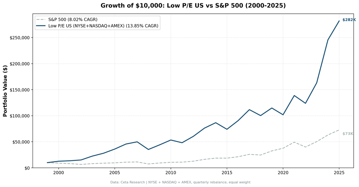
We backtested a low P/E value screen with quality filters across 25 years of US stock data (NYSE, NASDAQ, AMEX). 13.9% CAGR vs 8.0% for the S&P 500, with significant sector concentration in financials and energy.

Low P/E value investing has outperformed historically. Academic research going back to the 1970s documents the premium. But most investors use P/E wrong, and end up buying value traps instead of bargains. Here's how to screen for undervalued stocks while avoiding the traps.
Contents
- Method
- What Research Shows
- The Simple Screen
- The Advanced Screen
- Why Low P/E Works (And Why It Might Not)
- Why Quality Filters Matter
- What Historical Research Shows
- When It Works
- When It Fails
- Sector Concentration
- Rebalancing Frequency
- Limitations
- Implementation Tips
- Takeaway
- Part of a Series
- Run This Screen Yourself
- References
Data: FMP financial data warehouse, 2000–2025. Updated March 2026.
Method
Data source: Ceta Research (FMP financial data, 70K+ stocks) Universe: All US stocks with market cap > $1B Key metric: P/E ratio (trailing twelve months) Quality filters: ROE > 10%, Debt/Equity < 1.0
The screens below use current TTM data. For backtesting, you'd use historical data with proper point-in-time methodology (only using financial data that was available at the time of each simulated trade).
What Research Shows
Sanjoy Basu documented the low P/E premium in 1977. Stocks with low price-to-earnings ratios earned higher returns than expensive stocks, even after adjusting for risk. The pattern has been confirmed across multiple studies, time periods, and geographies.
But the path isn't smooth. Value strategies can underperform for extended periods. The 2010s were brutal: growth stocks dominated for nearly a decade. Many investors abandoned value strategies just before value sharply outperformed in 2022.
The premium exists. But capturing it requires patience most investors don't have.
The Simple Screen
Start with the basics. Find all stocks trading below a P/E of 15.
SELECT r.symbol, r.priceToEarningsRatioTTM, k.marketCap
FROM financial_ratios_ttm r
JOIN key_metrics_ttm k ON r.symbol = k.symbol
WHERE r.priceToEarningsRatioTTM > 0
  AND r.priceToEarningsRatioTTM < 15
  AND k.marketCap > 1000000000
ORDER BY r.priceToEarningsRatioTTM ASC
LIMIT 50
What this does: - priceToEarningsRatioTTM > 0 filters out money-losing companies (negative P/E) - priceToEarningsRatioTTM < 15 is the classic value threshold (below historical market average) - marketCap > 1000000000 ensures reliable data (no micro-caps)
This returns hundreds of stocks. Too many. Many are cheap for good reasons. We need quality filters.
The Advanced Screen
Add ROE and debt filters to avoid value traps.
SELECT
  r.symbol,
  r.priceToEarningsRatioTTM,
  k.returnOnEquityTTM,
  r.debtToEquityRatioTTM,
  k.marketCap
FROM financial_ratios_ttm r
JOIN key_metrics_ttm k ON r.symbol = k.symbol
WHERE r.priceToEarningsRatioTTM > 0
  AND r.priceToEarningsRatioTTM < 15
  AND k.returnOnEquityTTM > 0.10
  AND r.debtToEquityRatioTTM < 1.0
  AND k.marketCap > 1000000000
ORDER BY r.priceToEarningsRatioTTM ASC
LIMIT 50
New filters: - returnOnEquityTTM > 0.10 requires 10%+ return on equity. The company generates solid profits. - debtToEquityRatioTTM < 1.0 ensures conservative financing. Less bankruptcy risk.
This cuts the list from hundreds to about 50 stocks. That's the filter working. Value traps have low P/E but poor fundamentals. Genuine opportunities have low P/E with strong operations.
Why Low P/E Works (And Why It Might Not)
Sanjoy Basu first documented the low P/E premium in 1977. Stocks with low price-to-earnings ratios earned higher returns than expensive stocks, even after adjusting for risk. Lakonishok, Shleifer, and Vishny (1994) confirmed the finding across multiple valuation metrics. Fama and French (1992) documented a broader value premium using book-to-market ratios.
The pattern is robust. But researchers disagree on why.
Behavioral explanation: Investors overreact to bad news and ignore boring companies. Low P/E stocks are often companies that missed earnings, lost momentum, or operate in unfashionable sectors. The market overshoots to the downside. Patient buyers profit from the correction.
Risk explanation: Value stocks are genuinely riskier. They carry higher distress risk, more operating leverage, and greater sensitivity to recessions. The premium compensates investors for bearing real economic risk. Not a free lunch, but fair pay for a harder ride.
Both explanations likely capture part of the truth. What matters: the premium has persisted across decades and geographies.
Why Quality Filters Matter
A low P/E can mean two things: 1. The stock is undervalued (opportunity) 2. The stock is dying (trap)
ROE filters out struggling businesses. If a company can't generate decent returns on shareholder capital, it's probably cheap for a reason.
Debt filters out overleveraged companies. A stock might look cheap until you realize interest payments are crushing profits.
Without quality filters, you're buying a basket of cheap stocks. With them, you're buying a basket of cheap, profitable, well-financed stocks.
What Historical Research Shows
Multiple academic studies have examined low P/E returns:
Basu (1977): Found that low P/E stocks earned significantly higher returns than high P/E stocks in the 1957-1971 period, even after adjusting for beta risk.
Lakonishok, Shleifer, Vishny (1994): Studied value strategies from 1968-1990 using multiple metrics. The E/P (earnings-to-price) premium was approximately 4 percentage points annually. Using book-to-market ratios, value outperformed glamour by over 10% annually. Combined factor strategies showed a 7-9% gap. They attributed this partly to investor overreaction and extrapolation bias.
Fama & French (1992): Documented a broader value premium using book-to-market ratios. Their research showed that cheap stocks (by various metrics) systematically outperformed expensive stocks.
The premium has persisted across decades. But it comes with significant volatility and can disappear for years at a time.
When It Works
Low P/E value outperformed during:
2000-2002 (Tech Bubble Burst): Our backtest returned +26.6% in 2000 while SPY fell -10.5%. The strategy outperformed in all three dot-com crash years, producing a cumulative +85 percentage points of excess return from 2000-2002.
2003 (Post-Crash Recovery): Cheap stocks rebounded hard. The portfolio returned +48.8% in 2003, beating SPY by nearly 25 percentage points. Value picks that had been left for dead during the tech bubble came roaring back.
2022-2024 (Value Resurgence): Rising rates crushed growth stocks in 2022. Value held up better (-10.8% vs -19.0% for SPY). Then 2024 was the standout: the portfolio returned +50.5% vs SPY's +25.3%, a 25 percentage point gap. The broadest outperformance in the entire backtest.
Pattern: value works when expensive stocks get repriced. Crashes, rate hikes, and regime changes favor cheap stocks.
When It Fails
Low P/E value underperformed during:
2015 and 2019 (Growth Dominance): FAANG stocks drove returns. The portfolio lost -14.6% in 2015 while SPY was flat. In 2019, the portfolio gained +14.5% but SPY surged +32.3%, an 18 percentage point gap. When mega-cap growth runs, value can't keep up.
2020 (COVID Recovery): Our backtest returned -11.3% while SPY gained +15.6%, a 27 percentage point gap. Tech and growth led the rebound. Value missed the rally entirely.
Pattern: value struggles in momentum-driven bull markets. When investors chase growth, cheap stays cheap.
The late 2010s were tough. Growth dominance made value investing look broken. Many gave up. Those who held saw value outperform sharply from 2022-2024 when rising rates punished growth stocks and cheap stocks rallied.
Sector Concentration
Low P/E portfolios concentrate in specific sectors. Our backtest data shows the pattern:
- Financial Services: Over 50% of portfolio weight in mid-2022, consistently 35-50% from 2020-2023
- Energy: 40% in 2023-2024, 33% during the 2015 oil collapse
- Technology: Peaked at 23% in mid-2011 when tech valuations compressed
- Consumer Cyclical: 37% in 2017-2018
- Basic Materials: 20% in 2023
These sectors naturally trade at lower multiples. A P/E of 12 for a bank is normal. A P/E of 12 for a software company is a red flag.
This concentration creates risk. In 2008, financial services weight contributed to the -29.4% annual loss. In 2015, energy weight drove a -14.6% year. Sector-specific drawdowns hit value portfolios hard.
You're not just betting on "cheap stocks." You're often betting on specific sectors.
Rebalancing Frequency
Research generally supports infrequent rebalancing for value strategies.
Why? Transaction costs eat into returns. Frequent trading means paying spreads and commissions constantly. More importantly, value is a slow thesis. It takes time for the market to recognize that cheap stocks are undervalued.
Quarterly rebalancing aligns with earnings reporting cycles. You get fresh fundamental data, adjust positions, then hold. Annual rebalancing works too.
Daily rebalancing is counterproductive. You're paying transaction costs without new fundamental information to act on.
A note on costs: transaction costs varied significantly across our 2000-2025 backtest period. In the early 2000s, institutional trading costs ran 0.2-0.5%. By 2020, they dropped to near zero for retail investors. Our backtest uses a size-tiered cost model: 0.1% for large caps (>$10B), 0.3% for mid caps ($2-10B), and 0.5% for smaller stocks (<$2B). This better reflects the real cost of trading across the market cap spectrum.
Limitations
Universe: We test all US stocks (NYSE, NASDAQ, AMEX) with market cap > $1B. This includes companies across the full market cap spectrum above our floor, not just large-cap index members. The broader universe captures more value opportunities but also includes stocks with thinner liquidity. Survivorship bias is partially mitigated by FMP's inclusion of delisted companies, though coverage of delistings is less complete than active companies.
Point-in-time data: Proper backtests use quarterly reporting dates, but exact earnings release dates vary by company. Some firms report within 30 days of quarter-end, others take 60+. A conservative assumption is that data becomes available 45 days after the fiscal period end.
Sector concentration: The strategy naturally overweights cheap sectors. This isn't diversification. It's a sector bet.
No guarantee of future performance: The value premium existed historically. It may not continue. The late 2010s showed value can underperform for extended periods.
Implementation Tips
1. Be patient. Value can underperform for years. The 2010s proved that. You need conviction to hold through drawdowns.
2. Rebalance on schedule. Quarterly, not when it "feels right." Discipline beats emotion.
3. Watch sector exposure. If your portfolio is 40% financials, you're making a sector bet. Be aware.
4. Consider combining factors. Adding momentum or additional quality filters improves risk-adjusted returns.
5. Size positions appropriately. Value stocks can drop 30-50% and stay down. Don't bet more than you can stomach losing.
Takeaway
Low P/E value investing has worked historically. Academic research consistently shows a value premium across time periods and geographies. But "works" means over decades, not years. The strategy requires surviving extended drawdowns and underperformance cycles.
Most investors can't do it. They buy value after it rallies and sell after it underperforms. That's the opposite of what works.
The premium may persist because it's hard to capture. Patience and discipline are required. Most people lack both.
A note on data sources: The screens above use TTM (trailing twelve months) tables, which reflect current snapshots. The backtest numbers referenced in this article use historical tables (financial_ratios, key_metrics) with point-in-time methodology, only using data that was available at the time of each simulated trade. These are different data sources: TTM for live screening, historical for backtesting.
Data: Ceta Research (FMP financial data warehouse). Universe: NYSE + NASDAQ + AMEX, market cap > $1B. Screens use TTM tables. Backtest uses historical financial_ratios, key_metrics, and stock_eod tables with point-in-time methodology and 45-day reporting lag assumption. Transaction costs: size-tiered (0.1-0.5% one-way based on market cap). FMP data has known limitations: coverage varies by company and time period, some historical records may contain errors or gaps, and delisted company data is less complete than active companies. Past performance does not guarantee future results. This is educational content, not investment advice.
Part of a Series
This is the US analysis. We also ran the same screen on 12 global exchanges: - Low P/E on Indian Stocks (BSE + NSE) - 16.9% on BSE, 13.7% on NSE - Low P/E on Hong Kong Stocks (HKSE) - 14.4% CAGR, high volatility - Low P/E on UK Stocks (LSE) - 13.6% CAGR, +12.2% vs FTSE 100 - Low P/E Across 12 Global Exchanges - full comparison table
Run This Screen Yourself
Via web UI: Run the Low P/E screen on Ceta Research. The query is pre-loaded. Hit "Run" and see what passes today.
Via Python:
import requests, os

API_KEY = os.environ["CR_API_KEY"]
BASE = "https://api.cetaresearch.com/api/v1"

query = """
SELECT r.symbol, p.companyName,
    r.priceToEarningsRatioTTM as pe_ratio,
    k.returnOnEquityTTM * 100 as roe_pct,
    r.debtToEquityRatioTTM as debt_to_equity,
    k.marketCap / 1e9 as market_cap_billions
FROM financial_ratios_ttm r
JOIN key_metrics_ttm k ON r.symbol = k.symbol
JOIN profile p ON r.symbol = p.symbol
WHERE r.priceToEarningsRatioTTM > 0
    AND r.priceToEarningsRatioTTM < 15
    AND k.returnOnEquityTTM > 0.10
    AND r.debtToEquityRatioTTM >= 0
    AND r.debtToEquityRatioTTM < 1.0
    AND k.marketCap > 1e9
    AND p.exchange IN ('NYSE', 'NASDAQ', 'AMEX')
ORDER BY r.priceToEarningsRatioTTM ASC
LIMIT 30
"""

# Submit query
resp = requests.post(f"{BASE}/data-explorer/execute",
    headers={"X-API-Key": API_KEY, "Content-Type": "application/json"},
    json={"query": query, "options": {"format": "json", "timeout": 600}})
task_id = resp.json()["taskId"]

# Poll until complete
import time
while True:
    status = requests.get(f"{BASE}/tasks/data-query/{task_id}",
        headers={"X-API-Key": API_KEY}).json()
    if status["status"] in ("completed", "failed"):
        break
    time.sleep(2)

# Download results
results = requests.get(f"{BASE}{status['resultUrl']}",
    headers={"X-API-Key": API_KEY}).json()
for r in results[:10]:
    print(f"{r['symbol']:8s} P/E={r['pe_ratio']:.1f} ROE={r['roe_pct']:.1f}% D/E={r['debt_to_equity']:.2f}")
Get your API key at cetaresearch.com.
The full backtest code (Python + DuckDB) is available in our GitHub repository.
References
- Basu, S. (1977). "Investment Performance of Common Stocks in Relation to Their Price-Earnings Ratios." Journal of Finance, 32(3), 663-682.
- Fama, E. & French, K. (1992). "The Cross-Section of Expected Stock Returns." Journal of Finance, 47(2), 427-465.
- Lakonishok, J., Shleifer, A. & Vishny, R. (1994). "Contrarian Investment, Extrapolation, and Risk." Journal of Finance, 49(5), 1541-1578.